
Core Idea of OPT
📜 Statement of the Theory: What Does It Say, exactly?
Let’s begin with the core idea, as stated by the economists who formulated this theory:
“Given the natural resources, stock of capital, and state of technical knowledge, there will be a definite size of population that leads to the highest per capita income.”
If Question on OPT comes in exam, you can draw the following diagram:
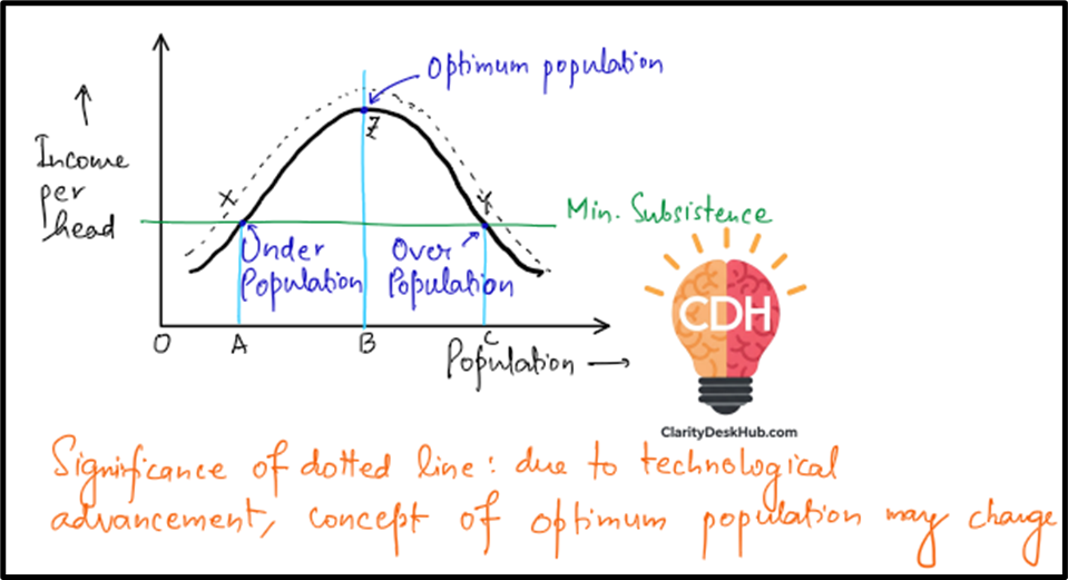
🌟 What Is Optimum Population?
Let’s get a bit more academic here:
🔹 Carl Saunders:
- Says optimum population is the one that produces maximum welfare—people are not just surviving, they are living well.
- Welfare includes health, education, jobs, and quality of life—not just income.
🔹 Prof. Edwin Cannan:
- Brings it down to return on labour.
- Think of labour as the number of workers in a field. If there are too few, the field isn’t fully farmed. If there are too many, they get in each other’s way.
- Optimum population, then, is that sweet spot where adding one more worker doesn’t increase output—in fact, output per person starts falling if we go beyond that.
🔹 Bounding:
- Puts it even more simply: optimum population is when standard of living is at its peak.
So, all three are basically saying the same thing—maximum output, efficiency, and well-being at a certain population level.
📉 Underpopulation
Now imagine a country has fewer people than its ideal population.
- There are lots of untapped resources—land, water, minerals—but not enough people to use them.
- This is like having 10 acres of farmland and only 2 farmers.
- Result? Low productivity, and thus, low per capita income.
➡️ Definition: If per capita income is low due to too few people, the country is underpopulated.
📈 Overpopulation
Now imagine the reverse.
- There are more people than resources can handle.
- It’s like 20 people trying to use 2 laptops in a cyber café.
- Everyone’s waiting, working inefficiently, and output per person drops.
➡️ Definition:
If per capita income is low due to too many people, the country is overpopulated.
So, remember:
Underpopulation = Too few people → Resources underutilized
Overpopulation = Too many people → Resources overstretched
Optimum population = Just right → Maximum per capita output
⚙️ Assumptions of the Optimum Population Theory
To make things simpler, the theory is based on a few key assumptions:
- Fixed Proportion of Working Population
- It assumes that the ratio of workers to total population (including children and elderly) stays constant as population grows.
- This is to avoid fluctuations in productivity due to changes in labour force.
- Fixed Natural Resources, Capital, and Technology
- No new land, no new machines, and no technological progress.
- This assumption helps in focusing purely on the impact of population changes, but in reality, this is a bit unrealistic, because we do invent better tools and discover new resources over time.
So, it’s a static model—useful for understanding concepts, but needs modifications to apply to real-world scenarios.
Let’s summarise a bit:
| Concept | Meaning | Impact on Per Capita Income |
|---|---|---|
| Optimum Population | Ideal number of people for max productivity | Highest |
| Underpopulation | Too few people to use resources fully | Lower |
| Overpopulation | Too many people straining limited resources | Lower |
In short, Optimum Population Theory gives us a framework to think about population not as a burden, but as a balancing act—where more is not always better, and less can be a problem too.
📊 Professor Dalton’s Formula: Measuring the Gap
Professor Dalton wanted to make the concept of optimum population more precise—not just a theoretical idea, but something we could measure.
So, he gave us a simple but powerful formula:
📐 Dalton’s Formula:
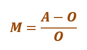
Where:
- M = Maladjustment (i.e., how far the current population is from the ideal one)
- A = Actual Population
- O = Optimum Population
🔎 How to Interpret It:
| Condition | Meaning |
|---|---|
| M = 0 | Perfect match → Optimum Population |
| M > 0 (Positive) | A > O → Overpopulation |
| M < 0 (Negative) | A < O → Underpopulation |
Let’s take a simple example. Suppose a country’s optimum population is 100 million.
- If actual population is also 100 million: M = (100−100)/100=0 ⇒ Optimum
- If population is 130 million: M = (130 – 100)/100 = 0.3 ⇒ Overpopulation
- If population is 80 million: M = (80 – 100)/100 = -0.2 ⇒ Underpopulation
🧠 Deeper Insight from Dalton:
He emphasized that optimum population is not a fixed number. It changes based on:
- Resources: New oil field? Higher optimum.
- Technology: Better farming tools? Higher optimum.
- Capital and knowledge: More schools, industries? Again, higher optimum.
👉 So, optimum population is relative, not absolute. It depends on the context of time, place, and development level.
🌍 Ackerman’s Population-Resource Regions: A Global View
Now let’s look at Ackerman, who introduced a more geographical perspective. He said:
“Don’t just talk about overpopulation or underpopulation in isolation. Look at the relationship between population, resources, and technology.”
He divided the world into five types of population-resource regions, based on how these three factors interact:
| Type | Resources | Technology | Population | Example |
|---|---|---|---|---|
| US Type | High | High | Optimum | United States |
| European Type | Low | High | High | Western Europe |
| Brazilian Type | High | Low | Low | Brazil |
| Egyptian Type | Low | Low | High | Egypt |
| Arctic Type | Low | Low | Low | Arctic regions (e.g., Greenland) |
🧭 Let’s Understand These Types One by One:
1. US Type (High Resources, High Technology, Optimum Population)
- Strong economy, advanced tech, rich in resources.
- People and resources are balanced → High productivity.
- Example: USA, Canada, Australia
2. European Type (Low Resources, High Technology, High Population)
- Fewer natural resources but compensated by technology.
- Think of countries like Germany or Japan—they import resources but produce a lot through skilled labour and tech.
3. Brazilian Type (High Resources, Low Technology, Low Population)
- Rich in land, water, and minerals—but low development.
- Underpopulated relative to potential.
- Example: Brazil, Congo Basin
4. Egyptian Type (Low Resources, Low Technology, High Population)
- Scarce resources, poor technology, yet very dense population.
- Pressure on limited land, leading to overpopulation.
- Example: Egypt, parts of Sub-Saharan Africa
5. Arctic Type (Low Resources, Low Technology, Low Population)
- Harsh climate, low resources, and very sparse population.
- Underpopulation, but potential also limited.
- Example: Arctic, parts of Siberia
🇮🇳 Where Does India Fit In?
India is partly Brazilian and mostly European type.
Why?
- We have some natural wealth (minerals, fertile plains) → Brazilian type.
- But we also have high population and limited per capita resources, balanced by growing technology → European type.
So, India’s challenge is to improve technology and capital investment, so that a large population becomes an asset, not a burden.
Let’s quickly revise what both gentlemen has to say:
- Dalton’s formula gives a mathematical way to measure how close or far a country is from its optimum population.
- Ackerman provides a global classification, reminding us that population issues vary based on local context—resources and technology both matter.
- India lies in a transitional category, with potential for improvement through investment in technology and resource management.