Köppen’s Climatic Classification

Whenever we study climate in geography, one question arises: how do we divide the Earth into meaningful climatic zones? Because climate is not just about temperature or rainfall alone. It affects vegetation, agriculture, lifestyle, even settlement patterns.

Now, among all climatologists, Vladimir Köppen — a Russian–German scientist — stands out. His classification is so successful that even today, more than a century later, the IPCC (Intergovernmental Panel on Climate Change) still uses it while predicting climate change up to the year 2100 CE. That itself shows the timelessness of his method.

📜 Historical Background

• Köppen was inspired by vegetation maps prepared by De Candolle. He believed that vegetation is the most visible expression of climate.
• He first published his map in the early 1900s, and then kept modifying it in 1918 and 1936.
• Later, Geiger (1954) refined it further, which is why you often hear the name Köppen–Geiger Classification.
• Interestingly, modifications have continued even in the 21st century (latest in 2018), proving how adaptable this framework is.

⚖️ Basis of Classification

Köppen did not depend only on one parameter. He used multiple criteria:

1. Vegetation correspondence – What kind of natural plants grow in that region.
2. Temperature of the warmest month & the coldest month – This helps differentiate between tropical, temperate, and polar regions.
3. Mean annual rainfall & rainfall of the driest month – To separate humid, semi-arid, and arid zones.

👉 Later revisions brought small modifications, but these three remain the foundation.

🏷️ Multi-Level Classification

Köppen’s brilliance lies in his multi-layered coding system. It is almost like giving an “address” to every climate region. Let’s decode this:

Level 1: Major Climatic Groups

He divided the world into five main climates.

• A, C, D, E → based on Temperature
• B → based on Precipitation

So:

• A = Tropical
• B = Dry/Arid
• C = Warm Temperate
• D = Cool Temperate
• E = Polar

Later in 1936, he added one more:

• H = Highland climates (based on Altitude).

Level 2: Seasonal Variations

Here, Köppen added symbols to show seasonality of precipitation and temperature. For example:

• f → no dry season
• s → dry summer
• w → dry winter

This made the classification more precise.

Level 3: Severity of Temperature / Continentality

At this stage, he distinguished hot vs cold within the same zone.

• h → hot
• k → cold

So, within the Dry Climate (B), you can have BSh (hot steppe) and BSk (cold steppe).

Level 4: Local Special Modifiers

Finally, Köppen acknowledged that some regions have unique features not captured by broad rules.

• g → Ganga type climate
• i → annual temperature range less than 5°C
• n → frequent fog

This fourth level adds the local touch, ensuring no special case is left out.

👉 So, to sum up: Köppen gave the world a four-level climatic “address system” — starting from broad groups, then seasonality, then severity, and finally local features. This system is still alive and evolving, just like our climate.

🌍 Köppen’s Classification (1900 onwards)

Level 1: The Five Major Climatic Groups (1900)

Köppen initially gave five groups of climates in 1900. Let’s decode them:

Symbol	Correspondence	Characteristics	Key Point
A	Tropical (Megatherms)	Uniform heat and abundant moisture.	Coldest month temp above 18°C.
B	Dry Climates	Xerophytic vegetation – long roots, thorns.	Evaporation > Precipitation.
C	Warm Temperate (Mesotherms)	Moderate heat and moisture.	Coldest month between –3°C & 18°C, warmest month ≥ 20°C.
D	Cold Snow Forest (Microtherms)	Plants adapted to low temp.	Coldest month ≤ –3°C; warmest month 10–22°C.
E	Polar (Hekistotherms)	Found in Arctic/Antarctic regions.	All months < 10°C.

📌 1936 Addition: Later, he added a sixth group –

• H = Highland Climates → Cold due to altitude (not latitude).

Level 2: Sub-Divisions (Seasonality of Rainfall/Temperature)

Now, within each major group, Köppen gave sub-types using small letters. These letters tell us about seasonality of rainfall.

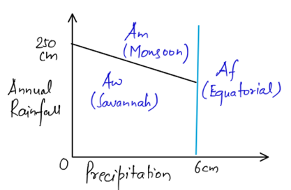
For Climate A (Tropical):

• f → Rainfall throughout the year (even driest month > 6 cm).
• w → Winter dry (e.g., Savannah grasslands).
• s → Summer dry (e.g., Tamil Nadu, because SW monsoon skips it).
• m → Monsoon type (excessive seasonal rainfall).

📌 Boundary Formula:

Where R = mean annual rainfall.
But this formula faced criticism: it was not scientifically accurate and seemed force-fitted.

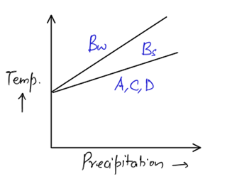
For Climate B (Dry):

• s → Semi-arid (Steppe)
• w → Arid (Desert)

📌 Boundary Formula:

Where P = precipitation limit; C = mean annual temperature (°C).

⚠️ Criticism: Sometimes this formula gave illogical results, suggesting uniform rainfall where it didn’t exist. Scholars believe Köppen drew graphs first, then fitted formulas later.

For Climate C (Warm Temperate – Mesothermal):

• f → Rainfall all year round (no dry season).
• w → Winter dry (driest winter month < wettest summer month).
• s → Summer dry (driest summer month ≤ 40 mm and ≤ 1/3rd of wettest month).

For Climate D (Cold Snow Forest – Microthermal):

• Same symbols as C (f, w, s) but applied to colder latitudes.

For Climate E (Polar):

• T = Tundra (warmest month 0–10°C).
• F = Frost/Ice-cap (warmest month < 0°C, leading to ice caps & permafrost).

📌 Note: H (Highland) has no sub-divisions in Köppen’s scheme.

Level 3: Sub-Divisions by Temperature Severity

Here, Köppen refined climates further with a, b, c, d, h, k type markers.

Climate Type	Sub-division	Characteristics
A	N.A.	Not Applicable.
B	h = hot	Mean annual temperature > 18°C.
	k = cold	Mean annual temperature < 18°C.
C	a	Warmest month temperature ≥ 22°C.
	b	Warmest month temperature < 22°C with at least 4 months above 10°C.
	c	Warmest month temperature < 22°C with at least 1–3 months above 10°C.
D	a, b, c	Same as C (applied to cold snow forest climates).
	d	Coldest month temperature < –38°C (Interior of the continents).
E & H	–	Not Applicable.

Level 4: Local Modifications

Finally, Köppen recognized some special local features and gave additional small letters:

• g → Ganga type climate (monsoon-dominated).
• i → Annual temperature range < 5°C.
• n → Frequent fog.
• n̄ → Infrequent fog.

🌟 Key Takeaway

• Level 1 = Broad groups (A to E + later H).
• Level 2 = Seasonality (f, w, s, m).
• Level 3 = Temperature severity (a, b, c, d, h, k).
• Level 4 = Local peculiarities (g, i, n).

👉 Thus, every climate type can be expressed with a unique “code”. For example:

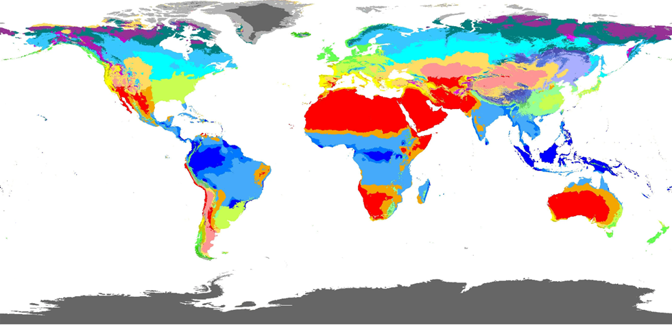
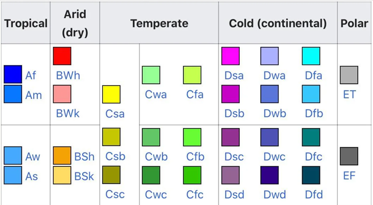
• Af = Tropical Rainforest (Amazon, Congo, Indonesia).
• Cfb = Warm temperate, rainfall all year, mild summers (British type climate).
• BWh = Hot desert (Sahara, Thar).
• ET = Tundra.

This “alphanumeric coding” is why Köppen’s classification is still the most widely used climatic system in geography.

Köppen Climatic Regions by Latitude

Latitude	Western Margin	Central (Continental)	Eastern Margin
90°	Polar (EF)
80°–65°	Tundra (ET)
65°–45°	British (Cfb)	Siberian (Dw)	Laurentian (Dfc)
45°–30°	Mediterranean (Cs)	Steppe (Bsh/Bsk)	China Type (Cfa)
30°–10°	Desert (BWh/BWk)	Savannah (Aw)	Monsoon (Am)
10° – 0° (Equator)	Equatorial (Af)

Tips to Remember:

• For 0, 90 and 80, polar, tundra and equatorial is obvious
• For Left side: you can remember: BMD
• For Center: Sib Stepped on Savanna (Here Sib= Lord Shiva)
• For Right: you can remember as: LCM
  
  Note: For 65°–45° latitudes, Precipitation (Rainfall/ Snowfall) in every month of year or throughout the year

Latitudinal Description:

• Polar + Tundra → Very less moisture, scanty precipitation. Albedo high (permafrost, no land for plants). Due to Earth’s tilt, long days of darkness/light. Vegetation: lichens, mosses. Found also over high mountains >4000m
• British (Cfb) – Deciduous type of forest, considered best climate of the world. Even rainfall, mild summers, cool winters (~13–18°C). Rainfall well-distributed; more rainfall in winter and autumn than summer/spring.
• Siberian (Dw) – Moisture throughout the year but very cold. Evergreen coniferous forest (taiga). Light rainfall in summer, snowfall in winter; Very low temperature, lowest inhabited climate; harshest climate for living
• Laurentian (Dfc) – Moderate summer rainfall, winter snowfall, mixed forest type vegetation.
• Mediterranean (Cs) – Dry hot summers, winter rainfall (25–35 cm, upto 55 cm too). Mediterranean forest with shrubs.
• Steppe (Bsh) – Temperate grasslands. Light summer rainfall, dry winters. Mostly arid/semi-arid.
• China Type (Cfa) – Heavy summer rainfall, deciduous forests, monsoonal effect.
• Desert (BWh) – Arid, low precipitation, xerophytic vegetation.
• Savannah/Sudan (Aw) – Grassland with trees + grasses. Distinct wet & dry season.
• Monsoon (Am) – Very heavy rainfall in summer, short dry winter. Dense tropical vegetation.
• Equatorial (Af) – Hot & wet throughout year. Evergreen rainforest.

Evaluating Köppen’s Climate Classification

Köppen’s system was one of the first serious attempts at classifying global climate in a structured way. Even today, it remains widely used, forming the basis for many modern climatic studies. However, like any pioneering work, it has its strengths and limitations.

🌟 Strengths of Köppen’s Classification

✅ Relevance

• The model is still relevant today; IPCC used it for climate prediction. The latest modification was in 2018.

✅ Universality

• Köppen’s Classification is applicable everywhere. Macro-level climate can be easily understood with its help.

✅ Simplicity and Clarity

• Köppen’s scheme uses easy-to-remember letter symbols (A, B, C, D, E) rather than long descriptive names.
• Even a beginner can quickly grasp the global climate zones without advanced meteorological knowledge.

✅ Strong Latitudinal and Zonal Control

• His classification clearly reflects how climate varies with latitude, making it easy to visualize the relationship between temperature, vegetation, and soils.
• This zonal approach makes climate distribution intuitive and predictable.

✅ Correlation with Vegetation and Biomes

• Köppen based his system on De Candolle’s vegetation maps, making a strong connection between climate and biomes.
• Even today, we often describe climates using vegetation terms:
  • Tropical rainforest (Af) 🌴
  • Boreal forests (Df, Dw) 🌲
  • Deserts and xerophytic vegetation (BW, BS) 🌵

✅ Flexibility and Adaptability

• Despite its empirical nature, Köppen’s system allows for local and seasonal variations, making it flexible.
• Later researchers have refined and expanded it without altering its core framework.

✅ Concept of Effective Precipitation

• His innovative formula for calculating effective precipitation (after accounting for evaporation) was a groundbreaking idea in climate science.
• It laid the foundation for later studies on aridity and water balance.

⚠️ Limitations and Criticisms of Köppen’s System

❌ Reverse Engineering Criticism

• Köppen correlated climate with vegetation, but critics argue this was not a true climatic analysis.
• Instead of objectively studying climate variables, he selected isotherms (temperature limits) based on vegetation boundaries, making it a descriptive system rather than a true climate theory.

❌ Oversimplification of Climate Controls

• Köppen’s system is primarily temperature-centric, with precipitation playing a secondary role.
• It does not consider:
  • Air masses
  • Wind patterns
  • Pressure belts
  • Ocean currents
  • Continentality and maritime influences

❌ No Differentiation Between Eastern and Western Coasts

• Köppen failed to distinguish between maritime and continental climates on the same latitude.
• Example:
  • The east coast of continents (humid summers) and the west coast (dry summers, maritime influence) are classified similarly, even though they have different climatic controls.

❌ Weak Treatment of Oceanic and Maritime Climates

• Köppen’s system largely ignores ocean currents, which are crucial in shaping coastal climates.
• He did not separately classify maritime vs. continental climates, overlooking insular climates (e.g., UK, Japan).

❌ Simplistic Approach to Precipitation

• While his effective precipitation concept was groundbreaking, it was too simplistic.
• Köppen did not fully consider all moisture losses, unlike Thornthwaite’s later concept of Potential Evapotranspiration (PET).

❌ Altitude ignored

• Though he modified his theory, Köppen failed to properly incorporate climatic variations due to altitude.

❌ Boundary Problem

• Boundaries of climatic regions were considered fixed, but in reality they are transitional in nature.

❌ Seasonality Issue

• His consideration of seasonal variation in temp. & rainfall led to debates, but he never explained the mechanism behind changes.

❌ Neglect of Microscale Studies

• Classification doesn’t provide idea of micro-scale or local-level climates (e.g., water balance, soil–climate relation).
• Example: São Paulo, Brazil
  • Köppen’s method identified only 26 micro-climates
  • Thornthwaite’s method identified 334 micro-climates.

🔍 Final Verdict: A Strong Yet Incomplete Framework

Köppen’s classification was a remarkable achievement for its time and is still used today due to its simplicity, clarity, and practical applications. However, it is more descriptive than explanatory, meaning it lacks deep scientific reasoning for why climates exist as they do.

👉 Modern climate classification systems, such as Thornthwaite’s, seek to improve upon Köppen’s model by incorporating factors like water balance, air masses, and ocean currents.

Yet, Köppen’s system remains a fundamental tool for anyone studying climate, geography, and ecology. It provides an excellent starting point for understanding Earth’s diverse climatic zones. 🌍