Weber’s Industrial Location Model

Imagine you are a businessman in the early 1900s, planning to set up an industry. The biggest question before you is: Where should I locate my factory so that the cost is minimum and profit is maximum?

This was the precise question that Alfred Weber, a German regional economist, attempted to answer in 1909 through his landmark theory known as:

Least Cost Location Theory, also known as Weber’s Industrial Location Model.

Let’s understand this theory:

🧠 Core Idea of Weber’s Theory

Weber believed that an industry should be located in such a place where the total cost—particularly transport cost—is the least. Therefore, his model is also called the Least Cost Theory.

At the heart of this theory is a variable cost analysis—where we study how costs like transport and labor change with location—and this is illustrated using a famous concept: Locational Triangle (we’ll come to that shortly).

🎯 Objectives of Weber’s Theory

Weber had two main objectives in mind:

1. To find the minimum cost location for setting up an industry.
2. To establish the centrality of transport cost in determining industrial location.

He believed that if we can minimize transport cost, we can maximize profit. Simple economics, right?

⚙️ Assumptions: The Ideal World of Weber

Like all classical theories, Weber’s model works under certain ideal conditions. These are like the rules of the game in his hypothetical model world. Let’s go through them:

1. Self-supporting Economy
   ➤ The region is economically self-contained and doesn’t depend on foreign trade.
2. Isotropic Surface
   ➤ The surface of the land is uniform in all directions—no mountains, rivers, or uneven terrain. Think of it like a blank, flat map.
3. Perfect Competition in the Market
   ➤ All firms are price takers; there’s no monopoly.
4. Static Labour & Uniform Wages
   ➤ Labour doesn’t move from place to place, and wages are the same across the region.
5. Socio-economic and Political Uniformity
   ➤ No regional variations in law, politics, or society. A utopian idea, but essential for a theoretical model.
6. Man is Rational and Economic
   ➤ Humans always act logically to maximize profit and minimize cost. (A classical economic assumption.)
7. Transport Cost Increases Uniformly
   ➤ Transport cost rises proportionately with distance and weight in all directions.
8. Uniform Demand, Uniform Price, Maximum Profit
   ➤ The product is equally demanded everywhere, sold at the same price, and earns maximum profit. Again, highly theoretical.

🧱 Types of Raw Materials in Weber’s Model

Weber emphasized that the type and nature of raw materials also influence industrial location. He classified them on two bases:

A. Based on Availability:

1. Ubiquitous Raw Materials
   ➤ These are available everywhere—like air, water, etc.
   ➤ For such materials, location doesn’t matter much.
2. Fixed (Localized) Raw Materials
   ➤ Found only in specific locations—like iron ore, coal, etc.
   ➤ Industries using these need to be closer to the source to reduce transport cost.

B. Based on Purity:

1. Pure Raw Materials (Non-weight-losing)
   ➤ The weight remains the same before and after processing.
   ➤ Example: Cotton in textile industry.
2. Impure Raw Materials (Weight-losing)
   ➤ Lose weight during processing.
   ➤ Example: Sugarcane (you get less sugar after crushing the bulky cane).

💡Implication: If a raw material is weight-losing, the industry should be located close to the source to save on transportation of bulky raw inputs.

So far, we have understood the what, why, and under what conditions of Weber’s Industrial Location Theory. The model is built around the idea that industries are economic entities, and hence their location is guided by a rational attempt to minimize cost—especially transport cost.

Next, we explore how Weber uses the concept of “Locational Triangle” to determine the actual placement of an industry on the map, and how labour and agglomeration factors later modify the basic transport-cost-based location.

🏭 Possible Locations of Industries (According to Weber)

Once Weber laid out the conditions and assumptions of his theory, he moved on to the practical question:

Where exactly should an industry be located to minimize cost?

He proposed that possible locations could be of two types:

1. Linear Location

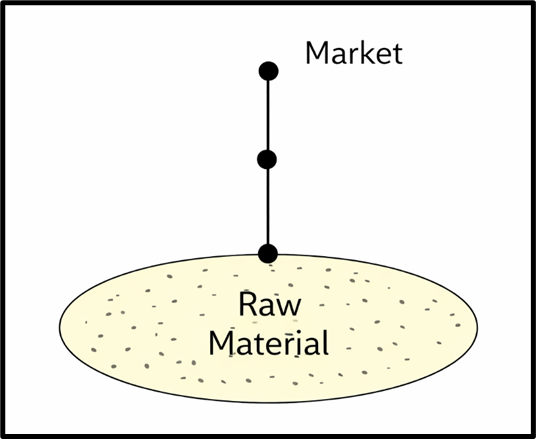
Think of this as a straight line between the market (M) and the source of raw material (R). The industry can be located at:

• The market
• The raw material source
• Or any point in between

But what determines the best point?

It all depends on the nature of raw material and the degree of weight loss during processing.

For example:

• Cotton textile industry – Cotton is fairly light and doesn’t lose much weight → often closer to market.
• Leather goods industry – Raw hides are bulky and lose weight during tanning → often closer to raw material source.

Hence, these industries follow a linear location pattern.

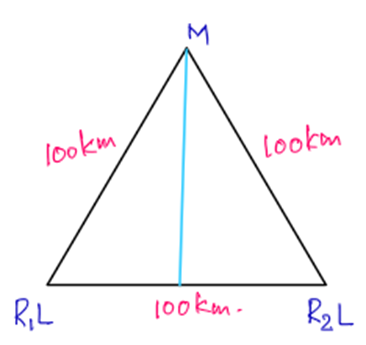
2. Non-Linear Location (The Triangle Model)

This is the heart of Weber’s theory—when two different raw materials are required from two different locations.

Here, the situation forms a triangle:

• Market (M)
• Raw material source R1
• Raw material source R2

Possible industry locations:

• At M, or
• At R1 or R2, or
• At any intermediate point between the three.

This is where three critical influences come into play:

🔁 Three Influences on Industrial Location

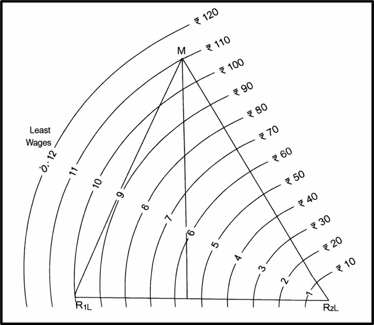
1. Influence of Transport Cost

Weber’s main argument: Industries locate where transport cost is minimized.

Let’s understand this through an example:

Assumptions:

• Two raw materials: R1 and R2.
• All three points (R1L, R2L, and M) form an equilateral triangle (each side = 100 km).
• R1L and R2L are localized and impure (they lose weight in processing).
• To produce 1 ton of finished goods, 2 tons of each raw material is required.
• Transport cost = Re 1 per ton per km.

Now let’s compute total cost for each location:

📍 Industry at R1L:

• Bring 2 tn of R2 = 2 × 100 × 1 = Rs. 200
• Deliver 1 tn product to market = 100 × 1 = Rs. 100
  👉 Total = Rs. 300

📍 Industry at R2L:

• Same as above → Rs. 300

📍 Industry at Market (M):

• Bring 2 tn from R1 + 2 tn from R2 = 4 × 100 = Rs. 400
  👉 Total = Rs. 400

📍 Industry at an Intermediate Point (I):

• Half distance from both → 50 km each for R1 and R2
• Transport cost = 2×50 + 2×50 = Rs. 200
• Product to market = 86.6 km (height of triangle) × 1 = Rs. 86.6
  👉 Total ≈ Rs. 286.6

✅ Conclusion: The intermediate location (I) is most economical.

2. Influence of Labour Cost

Weber understood that sometimes cheap labour could justify shifting the industry away from the least transport cost point.

He used the concept of:

🧭 Isotime –

A line joining points of equal additional transport cost from the least-cost location to the cheap labour centre.

Let’s understand with numbers:

• Transport cost at R2L = Rs. 250
• Labour cost = Rs. 500 (at R2L)
  👉 Total = Rs. 250 + Rs. 500 = Rs. 750

Now, suppose at point ‘O’,

• Extra transport = Rs. 100
• Labour cost = Rs. 350 (at point ‘O’)
  👉 Total = Rs. 250 + 100 + 350 = Rs. 700

✅ Even with higher transport, overall cost reduces, so point ‘O’ is better.

📌 Note: Earlier, unskilled labour couldn’t travel much due to high costs. Now, with improved transport, even unskilled labourers commute long distances, although skilled labour remains more mobile.

🌀 Isodapane –

• A line showing equal total transportation cost for raw materials + final product. It helps to find alternate locations where shifting is cost-effective.

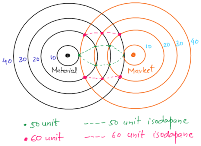
The diagram shows two fixed points: the Material Source located on the left (marked by a black dot) and the Market on the right (marked by an orange dot).

1. Around each of these points, concentric circles represent increasing transportation costs in units—10, 20, 30, and 40. The black circles surrounding the material source illustrate the cost of moving raw materials outward from the source, while the orange circles around the market indicate the cost of transporting the finished product toward the market.

Superimposed on the cost circles are isodapane lines, which are dashed lines representing points that incur the same total transportation cost (i.e., cost of raw material transport plus finished product transport).

• The green dotted line denotes the 50-unit isodapane, where each point reflects a combined transport cost of 50 units. These locations may serve as viable industrial sites if factors like labour or land cost are favourable enough to offset the slightly higher transportation expense.
• The pink dotted line signifies the 60-unit isodapane, representing locations where transport costs are higher and only become attractive if substantial non-transport savings—such as subsidies or drastically lower wages—exist.

Applying Weber’s theory to this diagram involves two steps:

• First, one must identify the least transport cost point, which typically lies somewhere between the material source and market—possibly near the overlap of the 10 and 20-unit rings—representing the optimum location for an industry from a pure transportation standpoint.
• Second, isodapanes are used to explore alternative sites. If, for example, labour is significantly cheaper on the 50-unit isodapane, and that saving exceeds the extra 10 units of transport cost, then it would be rational for the industry to shift there. Likewise, locations on the 60-unit isodapane could be selected if exceptional economic incentives justify the higher transportation burden.

3. Influence of Industrial Agglomeration

“Birds of the same feather flock together”—the same applies to industries.

When similar or complementary industries locate together, it leads to:

• Shared infrastructure
• Skilled labour pool
• Easy access to suppliers and buyers
• Reduced cost of production

This is called Industrial Agglomeration—a concept Weber acknowledged and modern geography strongly supports.

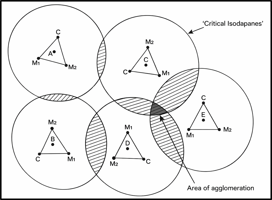
The diagram visually represents Alfred Weber’s concept of industrial agglomeration, which builds upon his theory of least-cost industrial location. It shows multiple locational triangles, each formed by two raw material sources (M₁ and M₂) and a market (C). Within each triangle, the points labeled A, B, C, D, and E indicate the least transport cost positions, which are Weber’s optimal locations for individual industries based on their own material-market geometry.

Surrounding each of these points are circles representing isodapane areas, or zones of relative cost-efficiency around the least transport cost point. These areas show where an industry could move slightly from the ideal point without drastically increasing its total transportation cost.

The most critical feature of the diagram is the overlapping shaded region where several of these isodapane zones intersect. This region marks the zone of agglomeration. Although it may not represent the absolute least-cost location for any single industry, it offers cumulative advantages for multiple industries locating together. These include shared infrastructure, labour pools, services, and reduced average transport costs due to proximity.

Thus, the diagram illustrates that even when individual industries have different optimal locations based purely on transport cost, they may still choose to cluster in a common zone. This shift is driven by the broader economic benefits of agglomeration, making such locations more favourable overall than isolated minimum-cost points. The shaded intersection symbolizes this practical compromise where collective savings from industrial clustering outweigh individual cost optimization.

⚖️ Criticism of Weber’s Theory

No theory is perfect, and Weber’s model too has limitations:

1. Freight rates are not always directly proportional to distance.
2. Rates for raw materials ≠ rates for finished goods.
3. It ignores demand-side factors—e.g., consumer preferences, market competition.
4. Too much reliance on idealistic assumptions (like isotropic surface, uniform wages).

Yet, we must credit Weber for emphasizing a fundamental economic logic:

✅ Transport cost matters most in industrial location decisions.

📌 Contemporary Relevance of Weber’s Theory

Despite being over a century old, Weber’s theory still holds value today:

1. Agro-based industries often still locate near villages to cut raw material and labour costs.
2. SEZs (Special Economic Zones) today are examples of industrial agglomeration—a direct echo of Weber’s idea.
3. Automobile industry is often located near markets (e.g., Detroit, Pimpri-Chinchwad) as finished goods are heavier than raw materials—this follows Weber’s logic.

✅ Conclusion

To sum up, Weber’s Industrial Location Theory is not just a theoretical model, but a rational framework for understanding how industries choose their locations based on minimizing cost, especially transport and labour costs, and sometimes agglomeration advantages.

It’s a classic example of how economic logic, when simplified and structured, can explain complex spatial decisions.